
Satu Mare
Satu Mare
Szatmárnémeti | |
|---|---|
 Left to right: Dacia Hotel, Firemen's Tower, Vécsey Palace (art museum), Roman Catholic Cathedral, Chain Church | |
 Location in Satu Mare County | |
 Satu Mare Location in Romania | |
| Coordinates: 47°47′24″N 22°53′24″E / 47.79000°N 22.89000°E | |
| Country | |
| County | Satu Mare |
| Status | County seat |
| Founded | 972 (first official record as Villa Zotmar) |
| Component villages | Sătmărel |
| Government | |
| • Mayor (2020–2024) | Gábor Kereskényi[1] (UDMR) |
| Area | |
| • Total | 150.3 km2 (58.0 sq mi) |
| Population (2021-12-01)[2] | |
| • Total | 91,520 |
| • Density | 669/km2 (1,730/sq mi) |
| Demonym(s) | sătmărean, sătmăreancă (ro), "szatmári","szatmárnémeti" (hu) |
| Time zone | UTC+2 (EET) |
| • Summer (DST) | UTC+3 (EEST) |
| Postal Code | 44xyz |
| Area code | +40 x61 |
| Car Plates | SM |
| Climate | Cfb |
| Website | www |
Satu Mare (pronounced [ˈsatu ˈmare] ⓘ; Hungarian: Szatmárnémeti [sɒtmaːrneːmɛti]; German: Sathmar; Yiddish: סאטמאר Satmar or סאַטמער Satmer) is a city with a population of 102,400 (2011). It is the capital of Satu Mare County, Romania, as well as the centre of the Satu Mare metropolitan area. It lies in the region of Maramureș, broadly part of Transylvania. Mentioned in the Gesta Hungarorum as castrum Zotmar ("Zotmar's fort"), the city has a history going back to the Middle Ages. Today, it is an academic, cultural, industrial, and business centre in the Nord-Vest development region.
Geography[edit]
Satu Mare is situated in Satu Mare County, in northwest Romania, on the river Someș, 13 km (8.1 mi) from the border with Hungary and 27 km (17 mi) from the border with Ukraine. The city is located at an altitude of 126 m (413 ft) on the Lower Someș alluvial plain, spreading out from the Administrative Palace at 25 October Square. The boundaries of the municipality contain an area of 150.3 square kilometres (58.0 sq mi).
From a geomorphologic point of view, the city is located on the Someș Meadow on both sides of the river, which narrows in the vicinity of the city and widens upstream and downstream from it; flooded during heavy rainfall, the field has various geographical configurations at the edge of the city (sand banks, valleys, micro-depressions).[3]
The formation of the current terrain of the city, dating from the late Pliocene in the Tertiary period, is linked to the clogging of the Pannonian Sea. Layers of soil were created from deposits of sand, loess and gravel, and generally have a thickness of 16 m (52 ft)–18 m (59 ft). Over this base, decaying vegetation gave rise to podsolic soils, which led to favorable conditions for crops (cereals, vegetables, fruit trees).[3]
The water network around Satu Mare is composed of the Someș River, Pârâul Sar in the north and the Homorod River in the south. The formation and evolution of the city was closely related to the Someș River, which, in addition to allowing for the settlement of a human community around it, has offered, since the early Middle Ages, the possibility of international trade with coastal regions, a practice that favored milling, fishing and other economic activities.[3]
Because the land slopes gently around the city, the Someș River has created numerous branches and meanders (before 1777, in the perimeter of the city there were 25 meanders downstream and 14 upstream). After systematisation works in 1777, the number of meanders in the city dropped to 9 downstream and 5 upstream, the total length of the river now being at 36.5 km (22.7 mi) within the city. Systematisation performed up to the mid-19th century configured the existing Someș riverbed; embankments were built 17.3 km (10.7 mi) long on the right bank and 11 km (6.8 mi) on the left. In 1970, the embankments were raised by 2 m (6.6 ft)–3 m (9.8 ft), protecting 52,000 hectares within the city limits and restoring nearly 800 ha of agricultural land that had previously been flooded.[3]
Flora and fauna[edit]
The flora associated with the town of Satu Mare is characteristic for the meadow area with trees of soft essence like wicker, indigenous poplar, maple and hazelnut. Grassland vegetation is represented by Agrostis stolonifera, Poa trivialis, Alopecurus pratensis and other types of vegetation.[3]
The city's largest park, the Garden of Rome, features some rare trees that are uncommon to the area, including the pagoda tree, native to East Asia (especially China); Pterocarya, also native to Asia; and Paulownia tomentosa, native to central and western China.[3]
Fauna is represented by species of rodents (hamster and european ground squirrel), reptiles, including Vipera berus in the Noroieni forest, and as avifauna species of ducks, geese, egrets, during passages and systematic occasional wanderings.[3]
Climate[edit]
Satu Mare has a continental climate, characterised by hot dry summers and cold winters. As the city is in the far north of the country, winter is much colder than the national average, with minimum temperatures reaching −17 °C (1 °F), lower than values recorded in other cities in western Romania like Oradea (−15 °C (5 °F)) or Timișoara (−17 °C (1 °F)). The average annual temperature is 9.6 °C (49 °F), or broken down by seasons: Spring 10.2 °C (50 °F), summer 19.6 °C (67 °F), autumn 10.8 °C (51 °F) and winter 1.7 °C (35 °F).[3] Atmospheric humidity is quite high. Prevailing wind currents blow in from the northwest, bringing spring and summer rainfall. Climate in this area has mild differences between highs and lows, and there is adequate rainfall year-round. The Köppen Climate Classification subtype for this climate is "Cfb" (Marine West Coast Climate/Oceanic climate).[4]
| Climate data for Satu Mare | |||||||||||||
|---|---|---|---|---|---|---|---|---|---|---|---|---|---|
| Month | Jan | Feb | Mar | Apr | May | Jun | Jul | Aug | Sep | Oct | Nov | Dec | Year |
| Mean daily maximum °C (°F) | 1 (34) |
3 (37) |
10 (50) |
15 (59) |
20 (68) |
22 (72) |
25 (77) |
25 (77) |
21 (70) |
15 (59) |
7 (45) |
2 (36) |
13 (55) |
| Mean daily minimum °C (°F) | −5 (23) |
−3 (27) |
1 (34) |
5 (41) |
9 (48) |
12 (54) |
13 (55) |
13 (55) |
10 (50) |
5 (41) |
0 (32) |
−2 (28) |
5 (41) |
| Average precipitation cm (inches) | 2 (0.8) |
2 (0.8) |
2 (0.8) |
4 (1.6) |
7 (2.8) |
8 (3.1) |
8 (3.1) |
7 (2.8) |
4 (1.6) |
4 (1.6) |
3 (1.2) |
2 (0.8) |
59 (23) |
| Source: weatherbase.com[5] | |||||||||||||
Name[edit]
The Hungarian name of the town Szatmár is believed to come from the personal name Zotmar, as the 13th-century Gesta Hungarorum gives the name of the 10th-century fortified settlement at the site of today's Satu Mare as castrum Zotmar ("Zotmar's fort").[6] The name Satu Mare, which means "great village" in Romanian, was used for the first time by the priest Moise Sora Novac in the 19th century.[7] An older Romanian name, Sătmar, was formally replaced by the current one in 1925.[8]
History[edit]


Archaeological evidence from Țara Oașului, Ardud, Medieșu Aurit, Homoroade, etc. clearly shows settlements in the area dating to the Stone Age and the Bronze Age. There is also evidence that the local Dacian population remained there after the Roman conquest in 101/106 AD. Later, these lands may have formed part of Menumorut's holdings; one of the important defensive fortresses – castrum Zotmar, dating to the 10th century – was at Satu Mare, as mentioned in the Gesta Hungarorum. After Stephen I of Hungary created the Kingdom of Hungary in the year 1000, German colonists were settled at the periphery of the city (Villa Zotmar), brought in by Stephen's wife, the Bavarian princess Gisela of Hungary. Later, they were joined by more German colonists from beyond the Someș River, in Mintiu.[9]
A royal free city since the 13th century, Satu Mare changed hands several times in the 15th century until the Báthory family took possession of the citadel in 1526,[10] proceeding to divert the Someș's waters in order to defend the southern part of the citadel; thus, the fortress remained on an island linked to the main roads by three bridges over the Someș. In 1562 the citadel was besieged by Ottoman armies led by Pargalı İbrahim Pasha of Buda and Maleoci Pasha of Timișoara. Then the Habsburgs besieged it, leading the fleeing Transylvanian armies to set it on fire. The Austrian general Lazar Schwendi ordered the citadel to be rebuilt after the plans of Italian architect Ottavio Baldigara; using an Italian system of fortifications, the new structure would be pentagonal with five towers.[9] After a period when it changed hands, the town came under Ottoman control in 1661. Called Sokmar by the new authorities, it was a kaza center within the Şenköy sanjak of Varat Eyalet. This status held until 1691, when the army of the Habsburgs expelled the Ottomans during the Great Turkish War.[11] In the Middle Ages, Satu Mare and Mintiu were two distinct entities.[9] The two settlements, then called "Szatmár" and "Németi", were united in 1715, and the resulting city was named "Szatmár-Németi".[12][13] On 2 January 1721, Emperor Charles VI recognised the union, at the same time granting Satu Mare the status of royal free city.[9] A decade earlier, the Treaty of Szatmár was signed in the city, ending Rákóczi's War for Independence.[14]
The city's importance was linked to the transportation and commerce of salt from nearby Ocna Dejului (Hungarian: Désakna, German: Salzdorf), possibly already at a very early date.[6] Due to the economic and commercial benefits it began to receive in the 13th century, Satu Mare became an important centre for craft guilds. In the 18th century, intense urbanisation began; several buildings survive from that period, including the old city hall, the inn, a barracks, the Greek Catholic church and the Reformed church. A Roman Catholic diocese was established there in 1804. In 1823, the city's systematization commission was established in order to direct its local government. In 1844, paving operations begun in 1805 were stepped up. The first industrial concerns also opened, including the steam mill, the brick factory, the Neuschloss Factory for wood products, the lumber factory, the Princz Factory and the Unio Factory. Due to its location at the intersection of commercial roads, Szatmárnémeti became an important rail hub. The line to Nagykároly (Carei) was built in 1871, followed in 1872 by a line to Máramarossziget (Sighetu Marmației) line, an 1894 link to Nagybánya (Baia Mare), 1900 to Erdőd (Ardud) and 1906 to Bikszád (Bixad).[9]
Since the second half of the 19th century, it underwent important economic and socio-cultural changes. The city's large companies (the Unio wagon factory, the Princz Factory, the Ardeleana textile enterprise, the Freund petroleum refinery, the brick factory and the furniture factory) prospered in this period, and the city invested heavily in communication lines, schools, hospitals, public works and public parks. The banking and commerce system also developed: in 1929 the chamber of commerce and industry, as well as the commodities stock market were established, with 25 commercial enterprises and 75 industrial and production firms as members. In 1930 there were 33 banks.[9]
After the collapse of Austria-Hungary, Romanian troops captured the town during their offensive launched on April 15, 1919.[15] By the Treaty of Trianon, Satu Mare officially ceased to be part of Hungary becoming part of Romania. In 1940, the Second Vienna Award gave back Northern Transylvania, including Satu Mare, to Hungary. In October 1944, the city was captured by the Soviet Red Army. After 1945, the city became again part of Romania. Soon afterwards, a Communist regime came to power, lasting until the 1989 revolution.[9]
Jewish community[edit]

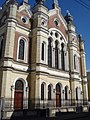
The presence of Jews in Transylvania is first mentioned in the late 16th century. In the 17th century, prince Gabriel Bethlen permitted Sephardi Jews from Turkey to settle in the Transylvanian capital Gyulafehérvár (Alba Iulia), in 1623.[16] In the early 18th century, Jews were allowed to settle in Sathmar. Some of them became involved in large-scale agriculture, becoming landlords or lessees, or were active in trade and industry,[17] or distilled brandy and leased taverns on crown estates. In 1715, when Sathmar became a royal town, they were expelled, beginning to resettle in the 1820s.[18] In 1841, several Jews obtained the permission to settle permanently in Sathmar; the first Jewish community was formally established in 1849, and in 1857, a synagogue was built. After a great number of traditional Ashkenazic Jews had settled in the town, the Jewish community split in 1898, when a supporter of the Hasidic movement was elected chief rabbi, into an Orthodox and a Status Quo community, led by a Zionist rabbi, which erected a synagogue in 1904.[17]
| Jewish population of Satu Mare | |||||||||||||
| Year | Jewish population (% of total population)[17][18] | ||||||||||||
|---|---|---|---|---|---|---|---|---|---|---|---|---|---|
| 1734 | 11 | ||||||||||||
| 1746 | 19 | ||||||||||||
| 1850 | 78 | ||||||||||||
| 1870 | 1,357 (7.4%) | ||||||||||||
| 1890 | 3,427 (16.5%) | ||||||||||||
| 1910 | 7,194 (20.6%) | ||||||||||||
| 1930 | 11,533 (21%) | ||||||||||||
| 1941 | 12,960 (24.9%) | ||||||||||||
| 1944 | ~20,000 | ||||||||||||
| 1947 | 5,000 to 7,500 | ||||||||||||
| 1970 | 500 | ||||||||||||
| 2011 | 34 | ||||||||||||
In the 1920s, there were several Zionist organizations in Satu Mare, and the yeshiva, one of the largest in the region, was attended by 400 students.[18] In 1930, the city had five large synagogues and about 20 shtiebels. In 1928, a conflict within the Orthodox community broke out over the election of a new chief rabbi, lasting six years and ending in 1934 with the appointment of the Hasidic rabbi Joel Teitelbaum, a traditionalist and anti-Zionist,[17] who later re-founded the Satmar Hasidic dynasty in Williamsburg, New York.[19][20] Another Hasidic rabbi, Aharon Roth, the founder of the Shomrei Emunim and Toldot Aharon communities in Jerusalem, was also active in Satu Mare.[18]
After Satu Mare became part of Hungary again in 1940, the civil rights and economic activities of the Jews were restricted, and in summer 1941, "foreign" Jews were deported to Kamenets-Podolski, where they were murdered by Hungarian and German troops.[17] In 1944, the Jewish population was forced into the Satu Mare ghetto; the majority of men were sent to forced labor battalions, and the others were deported to the extermination camps in Poland, where the majority of them were murdered by the Nazis.[18] Six trains left Satu Mare for Auschwitz-Birkenau, starting on May 19, 1944, each carrying approximately 3300 persons. The trains passed through Kassa (Košice) on May 19, 22, 26, 29, 30, and June 1.[21][22] In total, 18,863 Jews were deported from Satu Mare, Carei and the surrounding localities. Of these, 14,440 were killed.[23] Only a small number of the survivors returned to Satu Mare after the war, but a number of Jews belonging to linguistically and culturally different groups from all parts of Romania settled in the city. The majority of them later emigrated to Israel. By 1970, the town's Jewish population numbered 500,[18] and in 2011, only 34 Jews remained.[24]
In 2004, a Holocaust memorial was dedicated in the Decebal Street Synagogue's courtyard. Aside from the synagogues, two Jewish cemeteries also remain.[25]
Among the notable members of the local Jewish community have been historian Ignác Acsády, parliamentary deputies Ferenc Chorin and Kelemen Samu, politician Oszkár Jászi, writers Gyula Csehi, Rodion Markovits, Sándor Dénes, and Ernő Szép, painter Pál Erdös, Jacob Reinitz and director György Harag.[25]
Demographics[edit]
According to the 2021 census, Satu Mare had a population of 91,520, making it the 20th largest city in Romania.[26]
Religious composition of Satu Mare (2021)
| Year | Population | Romanians | Hungarians | ||||||||||
|---|---|---|---|---|---|---|---|---|---|---|---|---|---|
| 1880 | 7.9% | 83.1% | |||||||||||
| 1890 | 8.1% | 89.9% | |||||||||||
| 1900 | 7.8% | 89.01% | |||||||||||
| 1910 | 6.3% | 91.4% | |||||||||||
| 1920 | 15.2% | 63.6% | |||||||||||
| 1930 | 28.9% | 57.1% | |||||||||||
| 1941 | 6.6% | 90.2% | |||||||||||
| 1956 | 36.5% | 58.2% | |||||||||||
| 1966 | 44.2% | 54.9% | |||||||||||
| 1977 | 51.04% | 47.2% | |||||||||||
| 1992 | 55.8% | 43.2% | |||||||||||
| 2002 | 57.9% | 39.3% | |||||||||||
| 2011[24] | 58.9% | 37.6% | |||||||||||
| 2021 | 61.9% | 36.3% | |||||||||||
|
Source (where not otherwise specified): | |||||||||||||
Politics[edit]
.jpg)
Administration[edit]
The city government is headed by a mayor. Since 2016, the office is held by Gábor Kereskényi.[28] Decisions are approved and discussed by the local council made up of 23 elected councillors.[29] The city is divided into 12 districts laid out radially.[30] One of these, Sătmărel (Szatmárzsadány), is a separate village administered by the city.[31]
Additionally, as Satu Mare is the capital of Satu Mare County, the city hosts the palace of the prefecture, the headquarters of the county council and the prefect, who is appointed by Romania's central government. Like all other local councils in Romania, the Satu Mare local council, the county council and the city's mayor are elected every four years by the population.[32] The city is at the center of the Satu Mare metropolitan area, a metropolitan area established in 2013, with a population of 243,600, and which includes 26 cities, towns and communes.[33]
The Satu Mare City Council, elected at the 2020 local elections, is composed of the following parties:[34]
| Party | Seats in 2020 | Current Council | ||||||||||||
|---|---|---|---|---|---|---|---|---|---|---|---|---|---|---|
| Democratic Alliance of Hungarians in Romania (UDMR/RMDSZ) | 12 | |||||||||||||
| Save Romania Union (USR) | 4 | |||||||||||||
| National Liberal Party (PNL) | 4 | |||||||||||||
| Social Democratic Party (PSD) | 3 | |||||||||||||
The city day is 14 May, which commemorates the devastating floods that affected the city in 1970, although it is also a day of rebirth.
Justice system[edit]
Satu Mare has a complex judicial organisation, as a consequence of its status of county capital. The Satu Mare Court of Justice is the local judicial institution and is under the purview of the Satu Mare County Tribunal, which also exerts its jurisdiction over the courts of Carei, Ardud, Negrești-Oaș, Tășnad and Livada.[35] Appeals from these tribunals' verdicts, and more serious cases, are directed to the Oradea Court of Appeals.[36] Satu Mare also hosts the county's commercial and military tribunals.[35]
Satu Mare has its own municipal police force, Poliția Municipiului Satu Mare, which is responsible for policing of crime within the whole city, and operates a number of special divisions. The Satu Mare Police are headquartered on Mihai Viteazul Street in the city centre (with a number of precincts throughout the city) and is subordinated to the county's police inspectorate on Alexandru Iioan Cuza Street.[37] City Hall has its own community police force, Poliția Comunitară located on Universului Alley, dealing with local community issues. Satu Mare also houses the county's gendarmerie inspectorate.
Transport[edit]
Road[edit]
Satu Mare has a complex system of transportation, providing road, air and rail connections to major cities in Romania and Europe. The city is an important road and rail hub located near the borders with Hungary and Ukraine. The city is connected to other major Romanian cities by road (![]() European route E81,
European route E81, ![]() European route E671 and
European route E671 and ![]() European route E58) and by rail (CFR Main Line 400). The total number of automobiles registered in Satu Mare was 82,000 in 2008.[38] The city has around 400 streets with a total length of 178 km (111 mi) and cover an area of 1.3 km2 (0.50 sq mi).
European route E58) and by rail (CFR Main Line 400). The total number of automobiles registered in Satu Mare was 82,000 in 2008.[38] The city has around 400 streets with a total length of 178 km (111 mi) and cover an area of 1.3 km2 (0.50 sq mi).
Railway[edit]

Satu Mare Rail Station, located about 2 kilometres (1.2 mi) north of the city centre, is situated on the Căile Ferate Române Line 400 (Brașov – Siculeni – Deda – Dej – Baia Mare),[39] on Line 402 (Oradea – Săcueni – Carei – Satu Mare – Halmeu)[39] and on Line 417 (Satu Mare – Bixad).[39] CFR provides direct rail connections to all the major Romanian cities and to Budapest.[39] The city is also served by another secondary rail station, the Saw Station (Gara Ferăstrău).[39]
Public transport[edit]
The main public transportation system in Satu Mare consists of bus lines. There are twenty-three urban and suburban lines with a total length of 190.1 km (118.1 mi), the main operator being Transurban S.A.[40] In addition, there are various taxi companies serving the city. It is worth mentioning that Satu Mare had a trolleybus system in the past, created on the 15th of November 1994 but has been closed in 2005.
Airport[edit]
The city is served by the Satu Mare International Airport (IATA: SUJ, ICAO: LRSM), located 13 km (8.1 mi) south of the city, with a concrete runway, one of the longest in Romania, with TAROM and Wizz Air operating regular flights to Bucharest, London and Antalya (seasonal only).[41][42]
Sports[edit]
Football (soccer) is the most popular recreational sport in Satu Mare. There are two major football clubs in Satu Mare: Olimpia and Someșul Oar.[43] There are two football stadiums in Satu Mare: Stadionul Olimpia with 18,000 seats[44] and Someșul Stadium with 3,000 seats.
Other popular recreational activities include fencing, handball, bowling, women's basketball, karate and chess.
The local women's basketball team CSM Satu Mare is one of the best in the Romanian league; it finished third in the 2008/2009 season playoffs.[45] The team plays its home matches in the largest indoor arena in the city, the LPS Arena, which has a capacity of 400 seats.[44]
The Cypriot professional tennis player Marcos Baghdatis was brought to Satu Mare in 1998 for a month and a half by his former coach Jean Dobrescu[46] to train and to participate in local tennis competitions alongside his fellow Davis Cup team member, Rareș Cuzdriorean,[47] who is also a Satu Mare native with Cypriot citizenship.[48]
Fencing[edit]
Satu Mare has a tradition in fencing dating to 1885, and is the city that has supplied the most world and Olympic champions in Europe. Names like Ecaterina Stahl, Marcela Moldovan, Suzana and Ștefan Ardeleanu, Petru Kuki, Rudolf Luczki, Samuilă Melczhner, Geza Tere and in particular Alexandru Csipler figure prominently in the annals of Romanian fencing. The last four also formed the core of the city's fencing school, winning major local and international tournaments. Top results for which there is evidence date to 1935, when the local foil team, Olimpia Satu Mare, lost against CFR Timișoara by a score of 15–10 in the national final, while Rudolf Luczki won the sabre finals held in Cluj-Napoca. In 1973, the first signaling device in Romania was used in Satu Mare; this has been characterised as "a veritable revolution" for Romanian fencing.[49]
Economy[edit]

Satu Mare benefits from its proximity to the borders with Hungary and Ukraine, which makes it a prime location for logistical and industrial parks.
Companies that have established production facilities in Satu Mare are Voestalpine, Dräxlmaier Group,[50] Gotec Group,[51] Anvis Group,[52] Schlemmer, Casco Schützhelme and Zollner Elektronik[53][54] in the industrial sector; FrieslandCampina in the food sector; Radici Group in the textile sector; and Saint-Gobain and Boissigny in the wood industry.
Currently the largest private employer in Satu Mare is the German automotive company Dräxlmaier Group which owns since 1998 an electric engine components factory in the city and has around 3,600 employees. The factory supplies automotive wiring especially to the German car manufacturer Daimler AG but it also supplied wiring to another car manufacturer Porsche for its Porsche Panamera model.[55] The Swedish company Electrolux owns a kitchen stove factory in the city acquired in 1997, that has a surface area of 52,000 square metres (560,000 sq ft) and 1,800 employees. The facility has an annual production capacity of around 1.2 million units and the majority of the Zanussi brand kitchen stoves in Europe are manufactured there.[56][57] The Austrian company Voestalpine owns, since 2004, a steel tubes production facility with an annual capacity of 50 million units per year.[58] The German company Arcandor has its main Romanian office established in Satu Mare. The subsidiary, accounting for the region formed by Romania and Hungary, is the most important among the 16 subsidiaries in Europe in terms of the percentage of sales through online orders having in 2008 total orders of €19.3 million. The company also owns a 40,000 square metres (430,000 sq ft) logistic facility and a call center in the city.[59]
Satu Mare's retail sector is fairly well-developed; a number of international companies such as Carrefour, Auchan, Kaufland, Metro Point, Lidl and Penny Market have supermarkets or hypermarkets in the city. There is also a regional mall, Shopping City Satu Mare, with a gross leasable area (GLA) of 29,000 m2 (310,000 sq ft),[60] DIY stores (Dedeman, Brico Dépôt), and several other shopping centers: Grand Mall of 6,000 m2 (65,000 sq ft),[61] Plaza Europa of 3,000 m2 (32,000 sq ft)[62] and Someșul Mall, of 13,000 m2 (140,000 sq ft).[63]
There is also an industrial park called Satu Mare Industrial Park located at the edge of the city on a 70 ha surface.
Education[edit]
Universities[edit]

Satu Mare is home to the Commercial Academy of Satu Mare[64] and several other branches of important Romanian universities:
- Babeș-Bolyai University[64]
- Spiru Haret University[64]
- Technical University of Cluj-Napoca[64]
- University of Oradea[65]
- Vasile Goldiș West University of Arad[64]
High schools[edit]
Satu Mare has 16 high schools, of which four are national colleges:[66]
- Doamna Stanca National College[66]
- Ioan Slavici National College[66]
- Kölcsey Ferenc National College[66]
- Mihai Eminescu National College[66]
Gymnasiums[edit]
The city has 16 gymnasiums,[67] with the most important being:
- The Grigore Moisil Gymnasium (Școala Generală Grigore Moisil), founded in 1903 and named after the mathematician Grigore Moisil.[67][68]
- The Ion Creangă Gymnasium (Școala Generală Ion Creangă), founded in 1990 and named after the writer Ion Creangă.[67][69]
- The Lucian Blaga Gymnasium (Școala Generală Lucian Blaga), founded in 1996 by Ioan Viman and named after the philosopher and writer Lucian Blaga.[67][70]
Culture[edit]
Satu Mare has a county museum, an art museum,[71] and a theatre, the North Theatre, built in 1889 which has both a Hungarian and a Romanian section.[72] Concerts are given by the “Dinu Lipatti Philharmonic”, formerly the state symphonic orchestra of Satu Mare, in a concert hall in a wing of the Dacia Hotel.[73] The county library had 320.000 books in 1997, including a special bibliophile collections of over 70.000 volumes.[74]
Tourism[edit]

Major tourists attractions are:
- Administrative Palace, at 97 m (318 ft), one of the tallest buildings in Romania
- Capitoline Wolf statue
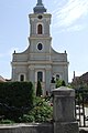
- Chain Church
- Dacia Hotel
- Decebal Street Synagogue
- Firemen's Tower, a 47 m (154 ft) tall tower
- Roman Catholic Cathedral
There are several hotels in the city: four 4-star hotels – Hotel Poesis, Villa Bodi, Satu-Mare City and Villa Class; eleven 3-star hotels – Astoria, Leon, Villa Lux, Dacia, Aurora, Dana I, Dana II, Select, Rania, Melody and Belvedere; and one 2-star hotel – Sport.
Media[edit]
Newspapers[edit]
- Informația Zilei – daily local newspaper[75]
- Gazeta de Nord-Vest – daily local newspaper[76]
- Cronica Sătmăreană – daily local newspaper
- Friss Újság – daily local newspaper in Hungarian language[77]
- Szatmári Magyar Hírlap – daily local newspaper in Hungarian language[78]
TV stations[edit]
Radio stations[edit]
Online portal[edit]
Consulates[edit]
 Honorary Consulate of Ukraine[79]
Natives[edit]
International relations[edit]
Twin towns and sister cities[edit]
Satu Mare is twinned with:
 Zutphen, Netherlands, since 1970[80]
 Wolfenbüttel, Germany, since 1974[81]
 Nyíregyháza, Hungary, since 2000[82]
- Berehove, Ukraine, since 2007[83]
 Rzeszów, Poland, since 2007[84][85]
Gallery[edit]
-
 Stephen the Great street
 -

-
-

-
-
 Hotel Dacia, detail


See also[edit]
- Satmar (Hasidic dynasty), a Jewish religious group named after this city
- List of companies based in Satu Mare
- List of natives and inhabitants of Satu Mare
References[edit]
- ^ "Results of the 2020 local elections". Central Electoral Bureau. Retrieved 8 June 2021.
- ^ "Populaţia rezidentă după grupa de vârstă, pe județe și municipii, orașe, comune, la 1 decembrie 2021" (XLS). National Institute of Statistics.
- ^ a b c d e f g h "Geografie" (in Romanian). www.satu-mare.ro. Archived from the original on June 12, 2009. Retrieved 2009-06-22.
- ^ "Climate Summary for Satu Mare". Weatherbase. Retrieved 2013-06-25.
- ^ "Weatherbase data for Satu Mare". Retrieved 2009-06-22.
- ^ a b Paul Niedermaier (2008). Städte, Dörfer, Bauwerke. Studien zur Siedlungs- und Baugeschichte Siebenbürgens (in German). Böhlau Verlag, Köln/Weimar. p. 320. ISBN 978-3-412-20047-3.
- ^ (in Romanian) Leontina Volosciuc, "Satu Mare: Oraș cu nume de sat și sat cu nume de oraș" ("Satu Mare: A City with the Name of a Village and a Village with the Name of a City"), Adevărul, 23 September 2010; accessed February 17, 2011
- ^ Attila Szabó (ed.), Erdély, Bánság És Partium Történeti És Közigazgatási Helységnévtára. Miercurea Ciuc, 2003, Pro-Print Könyvkiadó, ISBN 973-8468-01-9
- ^ a b c d e f g "History of Satu Mare City". Satu Mare City Hall. Retrieved 2013-06-29.
- ^ Paul Niedermaier (2008). Städte, Dörfer, Bauwerke. Studien zur Siedlungs- und Baugeschichte Siebenbürgens (in German). Böhlau Verlag Köln Weimar. p. 139. ISBN 9783412200473.
- ^ (in Turkish) Sadik Müfit Bilge, "Macaristan'da Osmanlı Hakimeyitinin ve İdari Teşkilatının Kuruluşu ve Gelişmesi", in OTAM (Ankara Üniversitesi Osmanlı Tarihi Araştırma ve Uygulama Merkezi Dergisi), vol. XI, p. 77, 2000
- ^ Ernst Hauler, Istoria nemților din regiunea Sătmarului, p.10. Editura Lamura, Satu Mare, 1998, ISBN 978-9739715-66-9
- ^ Judit Pál, "Administraţia şi elita oraşului Satu Mare în prima jumătate al secolului al XVIII-lea", in Laurenţiu Rădvan (ed.), Oraşul din spaţiul românesc între Orient şi Occident. Tranziţia de la medievalitate la modernitate., p.120. Editura Universităţii "Alexandru Ioan Cuza" din Iaşi, Iaşi, 2007, ISBN 978-973-703-268-3
- ^ Wandycz, Piotr Stefan. The Price of Freedom: A History of East Central Europe from the Middle Ages to the Present, p.85. Routledge, 2001, ISBN 0-415-25491-4
- ^ Béla Köpeczi (ed.). "History of Transylvania". Atlantic Research and Publications, Inc. Retrieved 2010-08-18.ISBN 0-88033-497-5
- ^ Patai, Raphael (1996). The Jews of Hungary. Wayne State University Press. pp. 154–161. ISBN 0-8143-2561-0.
- ^ a b c d e Marton, Yehouda, Schveiger, Paul (2007). "Satu-Mare". In Berenbaum, Michael; Skolnik, Fred (eds.). Encyclopaedia Judaica. Vol. 18 (2nd ed.). Detroit: Macmillan Reference. pp. 75–76. ISBN 978-0-02-866097-4.
{{cite encyclopedia}}: CS1 maint: multiple names: authors list (link) - ^ a b c d e f Tamás Csíki. "Satu Mare". The YIVO Encyclopedia of Jews in Eastern Europe.
- ^ Nathan, Joan (2006-12-13). "From Hungary, For Hanukkah, From Long Ago". The New York Times. Retrieved 2008-06-25.
- ^ Chris McKenna, "Satmar Grand Rebbe Moses Teitelbaum dies" Archived 2008-12-01 at the Wayback Machine, Record Online, 25 April 2006
- ^ "Death trains in 1944: the Kassa list" Archived 2012-03-30 at the Wayback Machine, National Committee for Attending Deportees
- ^ Tuvia Friling; Radu Ioanid; Mihail E. Ionescu, eds. (2004). International Commission on the Holocaust in Romania, Final Report (PDF). International Commission on the Holocaust in Romania; president of the commission: Elie Wiesel. ISBN 973-681-989-2. Archived from the original (PDF) on 2012-03-01.
- ^ "Let's not forget". www.jewishcomunity.ro. Retrieved 2009-06-14.
- ^ a b "Comunicat de presă privind rezultatele provizorii ale Recensământului Populaţiei şi Locuinţelor – 2011" (PDF). Satu Mare County Regional Statistics Directorate. 2012-02-02. Archived from the original (PDF) on 2013-10-29. Retrieved 2012-03-06.
- ^ a b "History". www.jewishcomunity.ro. Retrieved 2009-06-14.
- ^ "Rezultate definitive: Caracteristici etno-culturale demografice". Recensamantromania.ro. Retrieved 28 July 2023.
- ^ "Etnikai statisztikák" (in Hungarian). Árpád E. Varga. Retrieved 2009-06-13.
- ^ "Kereskényi Gábor (UDMR) a câștigat Primăria Satu Mare" (in Romanian). România Liberă. 2016-06-06. Retrieved 2016-06-15.
- ^ "Membri consiliul local" (in Romanian). www.satu-mare.ro. Retrieved 2009-06-13.
- ^ "Districts of Satu Mare" (in Romanian). Transurban. 2009-06-13. Archived from the original on 2012-02-13. Retrieved 2009-06-13.[better source needed]
- ^ "Urbanism, Satu Mare" (in Romanian). Satu Mare County Council. Archived from the original on September 25, 2010. Retrieved 2010-11-03.
- ^ "Law no. 215 / 21 April 2001: Legea administraţiei publice locale" (in Romanian). Parliament of Romania. Retrieved 2008-03-12.
- ^ "Vineri se constituie legal zona metropolitană Satu Mare" (in Romanian). Sătmăreanul. 2013-04-24. Retrieved 2013-05-20.
- ^ "Rezultatele finale ale alegerilor locale din 2020" (Json) (in Romanian). Autoritatea Electorală Permanentă. Retrieved 2020-11-02.
- ^ a b "Law no. 92 / 4 August 1992 for the judicial organisation" (in Romanian). Parliament of Romania. Retrieved 2008-03-12.
- ^ "Curtea de Apel Oradea" (in Romanian). Centrul Național de Informare Publică. Retrieved 2017-02-25.
- ^ "Law no. 218 / 23 April 2002: Law on the organisation and work of the Romanian Police" (in Romanian). Parliament of Romania. Retrieved 2008-03-12.
- ^ "Satu Mare: Mai multa poluare auto in municipiu" (in Romanian). neomania.ro. 2009-05-04. Retrieved 2009-06-03. [dead link]
- ^ a b c d e "Linii principale CFR" (PDF) (in Romanian). CFR.ro. 2009-06-03. Archived from the original (PDF) on 2007-09-27. Retrieved 2009-06-03.
- ^ "Linii urbane si sururbane" (in Romanian). Transurban. 2009-06-03. Archived from the original on 2009-05-22. Retrieved 2009-06-03.
- ^ Information about flights from/at LRSM (in Romanian)
- ^ Satu Mare Archived 2008-12-05 at the Wayback Machine (in Romanian)
- ^ "Turul Micula va juca în Liga a III-a pe Stadionul Olimpia" (in Romanian). www.informatia-zilei.ro. 2009-06-25. Archived from the original on 2009-06-28. Retrieved 2009-06-25.
- ^ a b Andrei Aricescu; Ecaterina Albici; Doru Radosav; Ovidiu Șerbănescu; Constantin Pohrib (1984). Ghid de oraș. Satu Mare (in Romanian). Satu Mare: Editura Sport-Turism.
- ^ "CSM Satu Mare" (in Romanian). www.numaibaschet.ro. 2009-05-21. Archived from the original on 2009-06-17. Retrieved 2009-05-21.
- ^ "Vedeta Australian Open s-a antrenat in Ardeal" (in Romanian). stiri.acasa.ro. 2006-01-25. Retrieved 2009-06-14.
- ^ "Campion in tara lui Marcos Baghdatis" (in Romanian). www.gazetanord-vest.ro. Archived from the original on 2009-06-14. Retrieved 2009-06-14.
- ^ "Un sătmărean în echipa de Cupa Davis a Ciprului" (in Romanian). www.satumareonline.ro. 2009-06-11. Retrieved 2009-06-14.
- ^ "Scurt istoric al scrimei sătmărene" (in Romanian). www.satu-mare.ro. 2009-05-21. Archived from the original on February 8, 2009. Retrieved 2009-05-21.
- ^ "Satu Mare". www.draexlmaier.de. Archived from the original on 2009-07-24. Retrieved 2009-06-23.
- ^ "Gotec Satu Mare". www.gotec-group.com. Archived from the original on 2011-07-11. Retrieved 2009-06-23.
- ^ "Anvis Satu Mare". www.anvisgroup.com. Retrieved 2009-06-23.
- ^ "Satu Mare plant 1". www.zollner.de. Archived from the original on 2009-05-12. Retrieved 2009-06-23.
- ^ "Satu Mare plant 2". www.zollner.de. Archived from the original on 2009-05-12. Retrieved 2009-06-23.
- ^ "De ce a concediat Draxlmaier 9.000 de angajaţi: "Avem nevoie de ingineri, nu de oameni mulți în producţie"". Ziarul Financiar. Retrieved 2010-08-24.
- ^ "Electrolux, primul an de scadere in Romania". Wall-Street (in Romanian). 2007-03-23. Retrieved 2009-10-23.
- ^ "Trei fabrici din Romania beneficiaza de credit cu buletinul". Cotidianul (in Romanian). 2006-03-19. Retrieved 2009-10-23.[permanent dead link]
- ^ "Harta marilor investiţii străine". Saptamana Financiara (in Romanian). 2008-05-16. Archived from the original on 2008-06-01. Retrieved 2009-10-23.
- ^ "Quelle, campioană la noi, pe butuci la nemţi". Adevarul (in Romanian). 2009-10-21. Archived from the original on 2009-10-23. Retrieved 2009-10-23.
- ^ "Mega mall-ul regional NEPI, deschis azi la Satu Mare" (in Romanian). Gazeta de Nord-Vest. Retrieved 2020-09-28.
- ^ "Grand Mall" (in Romanian). www.grand-mall.ro. Archived from the original on 2009-04-29. Retrieved 2009-06-23.
- ^ "Plaza Europa" (in Romanian). www.satu-mare.ro. Retrieved 2009-06-23.
- ^ "Centrul Comercial Someșul" (in Romanian). www.somesul.com.ro. Retrieved 2009-06-23.
- ^ a b c d e "Învăţământ superior" (in Romanian). www.satu-mare.ro. Retrieved 2009-06-29.
- ^ "Facultati/Universitati Satu Mare" (in Romanian). www.stirilocale.ro. Retrieved 2009-06-29.
- ^ a b c d e "Licee, Colegii" (in Romanian). www.satu-mare.ro. Archived from the original on 2017-06-30. Retrieved 2009-06-29.
- ^ a b c d "Școli" (in Romanian). www.satu-mare.ro. Retrieved 2009-06-29.
- ^ "ȘCOALA CU CLASELE I-VIII "GRIGORE MOISIL"" (in Romanian). www.satu-mare.ro. Retrieved 2009-06-28.
- ^ "ȘCOALA CU CLASELE I-VIII "ION CREANGĂ"" (in Romanian). www.satu-mare.ro. Retrieved 2009-06-28.
- ^ "SCURTĂ MONOGRAFIE" (in Romanian). www.l.blaga.go.ro. Archived from the original on 2008-12-01. Retrieved 2009-06-28.
- ^ "Museums". Satu Mare official website. Retrieved 2012-02-13.
- ^ "The North Theatre". Satu Mare official website. Retrieved 2012-02-13.
- ^ "Dinu Lipatti Philharmonic". Satu Mare official website. Retrieved 2012-02-13.
- ^ "The County Library". Satu Mare official website. Retrieved 2012-02-13.
- ^ "Informația Zilei" (in Romanian). www.mediaindex.ro. Archived from the original on 2012-02-24. Retrieved 2009-06-24.
- ^ "Gazeta de Nord-Vest" (in Romanian). www.mediaindex.ro. Archived from the original on 2012-02-24. Retrieved 2009-06-24.
- ^ "Friss Újság" (in Hungarian). www.mediaindex.ro. Archived from the original on 2009-01-30. Retrieved 2009-06-24.
- ^ "Magyar Hírlap" (in Romanian). www.mediaindex.ro. Archived from the original on 2012-02-24. Retrieved 2009-06-24.
- ^ "Consulat al Ucrainei la Satu Mare" (in Romanian). www.satumareonline.ro. 2008-10-03. Retrieved 2009-06-27.
- ^ "Zutphen – Olanda" (in Romanian). www.satu-mare.ro. Retrieved 2014-09-12.
- ^ "Wolfenbüttel – imaginea unui oraş" (in Romanian). www.satu-mare.ro. Retrieved 2014-09-12.
- ^ "Nyíregyháza – Ungaria" (in Romanian). www.satu-mare.ro. Retrieved 2014-09-12.
- ^ "Beregovo – Ucraina" (in Romanian). www.satu-mare.ro. Retrieved 2014-09-12.
- ^ "Rzeszow – Polonia" (in Romanian). www.satu-mare.ro. Retrieved 2014-09-12.
- ^ "Informacja o partnerstwie miast". www.rzeszow.pl. Retrieved 2014-09-12.
External links[edit]
Official websites[edit]
- Satu Mare administration official site (in Romanian, Hungarian, German, and English)
- Satu Mare County Prefecture (in Romanian)
- Satu Mare Municipal Council Archived 2022-08-16 at the Wayback Machine (in Romanian, Hungarian, German, and English)
- Transurban (Public Transport Company) official site (in Romanian)
- Satu Mare International Airport (in English and Romanian)
Unofficial websites[edit]
- Satu Mare Online (in Romanian)
- Satu-Mare.com (in Romanian)
- Szatmar.ro (in Hungarian)
Other[edit]
| Places of worship |  | |
|---|---|---|
| Historical buildings | ||
| Statues and monuments | ||
| Bridges | ||
| Sports venues | ||
| Other buildings | ||

County seats of Romania (alphabetical order by county) | ||
|---|---|---|
| ||
| International | |
|---|---|
| National | |
| Geographic | |